Traffic shaping with a RHEL Router
Traffic shaping is the ability to prioritize some traffic over others. Networks have limits and shaping gives you the ability to make choices about what traffic is most important when the demands for the network exceed these limits. With shaping you can choose to delay or drop lower priority traffic to ensure more important traffic flows unimpeded.
While it’s easy to understand the need for shaping and even how it works, its devilishly tricky to configure. The technology requires a network engineer understand queuing disciplines and how they impact networking. It gets more complex in the context of the Internet, where multiple devices are moving packets each with their own queue systems.
We’re going to cut through the complexity and look at a specific traffic shaping configuration that is suitable for most networks. We’ll take the code apart and provide enough explanation to ensure you can easily manage and modify it to suit your needs.
This article will develop and describe a script that can enable a Linux router to shape traffic between two networks. It was developed for Red Hat Enterprise Linux (RHEL) version 7.6, but it is compatible with any modern Linux. We’ll assume the following two network configuration.
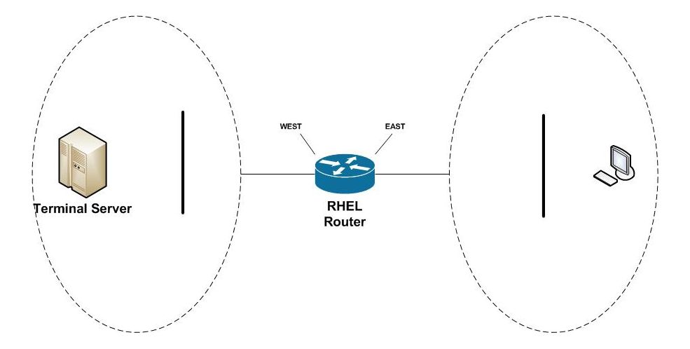
WEST and EAST are names assigned to Ethernet devices in our Red Hat router that connect the two networks. Users from the east network access the terminal server in the west network, along with other network services. We’re going to see how to prioritize terminal server traffic (TCP port 3389) over all others.
How to traffic shape in Red Hat
Traffic shaping in Red Hat is controlled through the tc(8) command which is part of the iproute2 project. tc(8) enables an engineer to perform a wide range of traffic control operations of which shaping is its most common use.
The traffic control system is built with three abstractions; qdiscs, classes and filters. We’re only going to discuss these briefly and provide just enough to understand our task at hand.
Qdiscs are queuing disciplines and they define the traffic control interface to the Linux system. It’s where packets enter into the traffic control system and leave on their way to the network device. There’s a large library of disciplines you can choose from, but we are going to focus on the two most important, tc-htb(8) and tc-sfq(8), which we’ll explain shortly.
Classes are where shaping take place. Classes give the power to delay, drop or even re-order packets and are heart of the queuing system. They introduce a hierarchical structure with parent classes flowing down to child classes. Its this structure that gives an engineer the power and flexibility to define queues and link them together.
Filters are how you direct packets into classes. Qdiscs will define a default path that is followed unless a filter overrides that path. By overriding the path an engineer can direct a packet to a class which can then shape the traffic. Filters provide a flexible pattern matching system to identify packets of interest and to then classify them.
Caveats
There are two important caveats to be mindful of when working with traffic shaping. The first is that you can only shape outbound (e.g. egress) traffic. To address this limitation and ensure our priorities are applied to all network traffic, we create two queues, one on our WEST network interface and one on our EAST.
The second caveat deals with how we manage speeds when a router is connected to networks of different abilities. For example, we will assume the router’s WEST network interface is a 20 Mbps (megabits) Internet connection and it’s EAST network interface is a 100 Mbps LAN network. We must limit the flows to the slowest link otherwise the faster network could overwhelm the slower and our shaping would have no effect. To ensure that our shaping is enforced, we’ll speed limit both WEST and EAST to 20 Mbps.
The Code
What follows is a bash script to create our traffic shaping policy.
#!/bin/bash

configure() {
    local device=$1
    local maxrate=$2
    local limited=$3

    # Delete qdiscs, classes and filters
    tc qdisc del dev $device root 2> /dev/null

    # Root htb qdisc -- direct pkts to class 1:10 unless otherwise classified
    tc qdisc add dev $device root handle 1: htb default 10

    # Class 1:1 top of bandwith sharing tree
    # Class 1:10 -- rate-limited low priority queue
    # Class 1:20 -- maximum rate high priority queue
    tc class add dev $device parent 1: classid 1:1 htb rate $maxrate burst 20k
    tc class add dev $device parent 1:1 classid 1:10 htb \
        rate $limited ceil $maxrate burst 20k
    tc class add dev $device parent 1:1 classid 1:20 htb \
        rate $maxrate ceil $maxrate burst 20k

    # SFQ ensures equitable sharing between sessions
    tc qdisc add dev $device parent 1:10 handle 10: sfq perturb 10
    tc qdisc add dev $device parent 1:20 handle 20: sfq perturb 10

    # Classify ICMP into high priority queue
    tc filter add dev $device parent 1:0 protocol ip prio 1 u32 \
        match ip protocol 1 0xff flowid 1:20

    # Classify TCP-ACK into high priority queue
    tc filter add dev $device parent 1: protocol ip prio 1 u32 \
        match ip protocol 6 0xff \
        match u8 0x05 0x0f at 0 \
        match u16 0x0000 0xffc0 at 2 \
        match u8 0x10 0xff at 33 \
        flowid 1:20
}

main() {
    # Enable rate reporting in the htb scheduler
    echo 1 > /sys/module/sch_htb/parameters/htb_rate_est

    configure WEST 20mbit 5mbit
    configure EAST 20mbit 5mbit

    # Classify terminal server traffic outbound to WEST
    tc filter add dev WEST protocol ip parent 1: prio 2 u32 \
        match ip dport 3389 0xffff flowid 1:20

    # Classify terminal server traffic outbound to EAST
    tc filter add dev EAST protocol ip parent 1: prio 2 u32 \
        match ip sport 3389 0xffff flowid 1:20
}

main "$@"
The explanation
Lines 3 through 39 define the configure() function. This is where we build an egress queue for a specific Ethernet device. The function accepts three parameters; the device name, the maximum speed we want to allow outbound for the device and the lower speed we want to use for our low priority traffic. Before we delve into the details, let’s talk about the speeds and how we intend for them to be used.
Our traffic shaping system is built upon a queuing system called “Heirarchical Token Bucket” or HTB. It’s a clever technology that enables us to build a pyramid of priorities. We use this pyramid system to define two queues; a high priority queue and a low priority queue. We are going to put our terminal server traffic into the high priority queue and everything else into the low priority queue.
What’s particularly clever about the HTB system is each level of the hierarchy allows bandwidth “borrowing” of unused capacity. The idea is if the high priority queue doesn’t use all of it’s allotment, the low priority queue can have it. You can read more about HTB at tc-htb(8).
# Root htb qdisc -- direct pkts to class 1:10 unless otherwise classified
tc qdisc add dev $device root handle 1: htb default 10
Lines 12 creates the root queue for each Ethernet device. As the name root implies, it is the top of our queue hierarchy. It’s where packets are added by the kernel and removed by the device. The thing to keep in mind — the root is where packets leave the queue. They don’t “fall off” the bottom of the hierarchy. It’s the moving down and back up again that allows borrowing to take place.
Line 12 also establishes an important default. The suffix default 10 configures the packet flow to use the queue id 1:10. Unless a filter interferes, this is the default path which is the low priority queue.
# Class 1:1 top of bandwith sharing tree
# Class 1:10 -- rate-limited low priority queue
# Class 1:20 -- maximum rate high priority queue
tc class add dev $device parent 1: classid 1:1 htb rate $maxrate burst 20k
tc class add dev $device parent 1:1 classid 1:10 htb \
    rate $limited ceil $maxrate burst 20k
tc class add dev $device parent 1:1 classid 1:20 htb \
    rate $maxrate ceil $maxrate burst 20k
Line 17 creates a class directly beneath the root with the id 1:1. This defines the maximum bandwidth available for all sub-queues below it.
Line 18 defines our low priority queue with the id 1:10. The use of the ceil parameter defines how much it can borrow from the parent. We set it to borrow as much spare bandwidth the parent has available
Line 20 defines our high priority queue with the id 1:20. This queue has the same rate as it’s parent and is therefore allocated the full rate available.
An interesting behavior develops if both the low priority and high priority queue are competing for bandwidth. The queuing system allots capacity based on their ratio of speed allocation. Because we are planning to allocate 20 Mbps for the high priority queue and 5 Mbps for the low priority queue the allocation will be 4-to-1. That means 4 packets for the high priority queue for every 1 packet to the low priority queue.
# SFQ ensures equitable sharing between sessions
tc qdisc add dev $device parent 1:10 handle 10: sfq perturb 10
tc qdisc add dev $device parent 1:20 handle 20: sfq perturb 10
Lines 24 and 25 define two SFQ queues for the bottom of our hierarchy. SFQ doesn’t do any shaping, but instead uses a round-robin scheduling system that ensures each “flow” gets a fair chance to send packets. In this context, a flow corresponds to a TCP/IP connection and SFQ ensures one connection can’t monopolize the bandwidth. You can read more about SFQ at tc-sfq(8).
# Classify ICMP into high priority queue
tc filter add dev $device parent 1:0 protocol ip prio 1 u32 \
    match ip protocol 1 0xff flowid 1:20
Line 28 introduces our first filter. This filter looks for ICMP traffic (e.g. ping packets) and directs them to the high priority queue. This ensures that even during periods of heavy network use, engineers still have the ability to use ping for diagnostics.
# Classify TCP-ACK into high priority queue
tc filter add dev $device parent 1: protocol ip prio 1 u32 \
    match ip protocol 6 0xff \
    match u8 0x05 0x0f at 0 \
    match u16 0x0000 0xffc0 at 2 \
    match u8 0x10 0xff at 33 \
    flowid 1:20
Line 32 is another filter. This one directs TCP-ACK packets into the high priority queue. Doing so ensures timely delivery of these important communication acknowledgements, even if the network is experiencing heavy use. If ACKs are delayed too long, a sender could interpret it as a drop and resend the original sequence, further increasing network load.
Lines 40 through 54 defines the main() function. This is the starting point for the script and causes the configuration of the queues.
# Enable rate reporting in the htb scheduler
echo 1 > /sys/module/sch_htb/parameters/htb_rate_est
Line 42 enable rate reporting of queues. This is a useful feature that allows an engineer to monitor traffic shaping system performance. We’ll provide some examples shortly.
configure WEST 20mbit 5mbit
configure EAST 20mbit 5mbit
Lines 44 and 45 configure our two network interfaces by invoking the configure() function already describe.
# Classify terminal server traffic outbound to WEST
tc filter add dev WEST protocol ip parent 1: prio 2 u32 \
    match ip dport 3389 0xffff flowid 1:20

# Classify terminal server traffic outbound to EAST
tc filter add dev EAST protocol ip parent 1: prio 2 u32 \
    match ip sport 3389 0xffff flowid 1:20
Line 48 defines the egress filter for the WEST Ethernet interface. It directs packets with a destination port of 3389 into the high priority queue.
Line 52 defines the egress filter for the EAST Ethernet interface. It is similar to the WEST egress, but it direct packets with a source port of 3389 into the high priority queue.
Monitoring traffic shaping
The simplest way to monitor the traffic shaping system is with the tc(8) command. The following two commands will report the statistics of the WEST and EAST interfaces respectively.
# tc -s class ls dev WEST
# tc -s class ls dev EAST
The output of each will look similar. Here is a sample taken from a live system using the traffic control script. The yellow highlighted sections identify the most important elements to watch.
class htb 1:10 parent 1:1 leaf 10: prio 0 rate 5Mbit ceil 20Mbit burst 20Kb cburst 1600b
 Sent 18575133765 bytes 28631268 pkt (dropped 111212, overlimits 0 requeues 0)
 rate 273688bit 122pps backlog 0b 0p requeues 0
 lended: 21760240 borrowed: 6871028 giants: 0
 tokens: 509550 ctokens: 9387

class htb 1:1 root rate 20Mbit ceil 20Mbit burst 20Kb cburst 1600b
 Sent 34359166476 bytes 155788322 pkt (dropped 0, overlimits 0 requeues 0)
 rate 905232bit 1110pps backlog 0b 0p requeues 0
 lended: 6871028 borrowed: 0 giants: 0
 tokens: 127243 ctokens: 9243

class htb 1:20 parent 1:1 leaf 20: prio 0 rate 20Mbit ceil 20Mbit burst 20Kb cburst 1600b
 Sent 15784032711 bytes 127157054 pkt (dropped 610, overlimits 0 requeues 0)
 rate 631544bit 987pps backlog 0b 0p requeues 0
 lended: 127157054 borrowed: 0 giants: 0
 tokens: 127243 ctokens: 9243
The output is broken into three sections, one for each of our three classes. Each section identifies the class, it’s configuration and the statistics it’s collected since it was created.
The top of the class hierarchy is class 1:1. It’s useful to watch these statistics to get an overview of the total packets flowing through the system. The most useful statistics are the rate which is the bits per second of packets flowing outbound and the pps which is the packets per second.
Watching the individual queues also are useful to get a sense of how the network is being used. You can refresh the report and compare successive invocations to see how the queues are being allocated packets.
A useful way to watch the queues in real time is to combine one of these commands with the watch(1) utility. For example:
# watch tc -s ls dev WESTYou should watch for excessive dopped packets or periods where an individual queue is sustaining it’s maximum allocation. Either of these can indicate your network is exceeding it’s capacity. You can use this to guide modifications to your queue configuration or to investigate the cause – perhaps it’s an indication of rogue traffic or network misuse. If your network is dropping excessive packets or sustaining it’s maximum capacity for prolonged periods of time, you will need to take action and these statistics give you what you need to know.
Summary
Armed with this script you can precisely control how your network prioritizes traffic. You’ll find with it, you can accomplish 90% of your needs with little to no modifications.
The tc(8) system is an impressive technology with a dizzying array of options. The best advice when testing it’s capabilities is to experiment in a lab. It’s simple to build a network lab using widely available VM technology such as VirtualBox, Xen and Hyper-V. Tools such as netcat and iperf are excellent at generating almost any traffic flow you need.
Carroll-Net was founded in 1994 with the singular goal of providing datacenter services our clients require at a price they can afford, delivered everywhere they need them. The industry now calls this cloud services — we call it common sense.
You might like some of our other articles…
 Red Hat Bare Metal Backups |  Red Hat Dynamic Routing |  Image vs. File Backups | Tools for Tracking Hackers |